Examples
Where the cubesat designs come from
The case is a fleet of identical 12U-class cubesats whose power, mass and attitude control are coupled, described by a SysML v2 system model. A configuration swaps the reaction wheel and the star tracker, tunes the panel span, the battery capacity and the controller gains Kp and Kd, and sets the fleet size; the slew is simulated and the model computes the rest. A row is one synthetic design. Two regimes of 3,000 designs differ in the sampled gains. The model and the data are in examples/adcs/:
uv run python examples/adcs/k_terms.py
What each column measures
metric (orientation)           unit      column
settling time (-1)             s         settling_time_s
pointing error (-1)            deg       pointing_error_deg
total mass (-1)                kg        total_mass_kg
control effort (-1)            N.m.s     control_effort
power margin (+1)              W         power_margin_w
energy balance (+1)            Wh        energy_balance_wh
peak slew power (-1)           W         peak_slew_power_w
depth of discharge (-1)        fraction  dod_eclipse
momentum headroom (+1)         ratio     momentum_headroom
available power (+1)           W         available_power_w
battery peak power ratio (+1)  ratio     battery_peak_power_ratio
unit cost (-1)                 USD       unit_cost_usd
fleet cost (-1)                USD       fleet_cost_usd
configuration: wheel class, star-tracker grade, panel span,
  battery capacity, Kp, Kd, fleet size
Thirteen metrics are traded. Pointing error, unit cost and fleet cost are the stakeholders' measures of effectiveness; the other ten are measures of performance. Orientation -1 marks a cost, inverted. With four feasibility flags on settling, momentum, power and depth of discharge, the primary regime has 2,134 feasible designs of 3,000.
What the fit is asked
The stakeholders ask for a payload that points and a fleet they can afford. Near the frontier, do their three measures trade against one another and against the subsystems' measures, and does one trade describe the table, or two?
The one-term fit
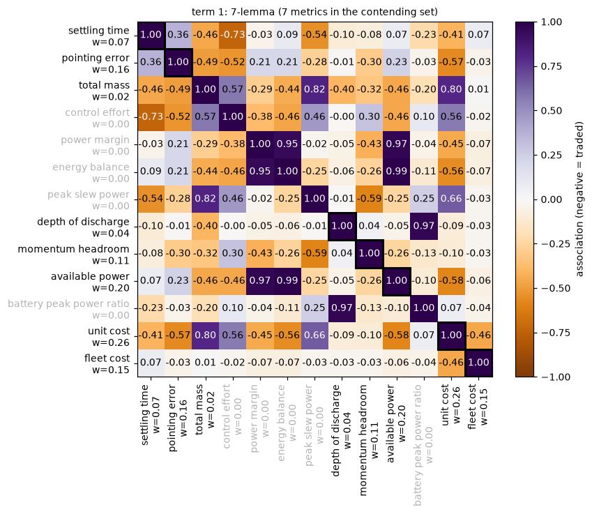
At the fit temperature select_temperature picks for a tenth of designs above V = 1, the one-term trade-off report finds a contending set of seven metrics that trade off, a 7-lemma: unit cost, available power, pointing error, fleet cost, momentum headroom, settling time, depth of discharge.
import sys

sys.path.insert(0, "examples/adcs")
import case

study = case.load_study("primary")
fit = case.fit_study(study, K=1)
case.association_figure(study, fit)
Choosing K on the case
The choosing-K checks on both regimes, each at its K = 1 temperature (recipe).
import numpy as np
from tradespace import HyperbolicTradeSpace


def fit_k(M, K, tau, seed=0):
    return HyperbolicTradeSpace(
        n_terms=K, temperature=tau, random_state=seed
    ).fit(M)


def sweep(M, tau, Ks):
    """One line per K at one temperature; returns the mean slacks."""
    slack = []
    for K in Ks:
        fit = fit_k(M, K, tau)
        t = fit.termination_
        print(
            f"K={K} slack={fit.mean_slack_:.3f}"
            f" thinnest={fit.term_share_.min():.2f}"
            f" {t.status} radius={t.radius:.0e}"
        )
        slack.append(fit.mean_slack_)
    print("drops", -np.diff(slack).round(3))
    return np.array(slack)


def movement(M, K, tau, draws=2, seed=0):
    """Largest distance to the nearest term of a refit on a resample."""
    ref = fit_k(M, K, tau)
    rng = np.random.default_rng(seed)
    moved = np.zeros(K)
    for s in range(draws):
        W = fit_k(M[rng.choice(len(M), len(M))], K, tau, s).exponents_
        d = np.abs(W[:, None] - ref.exponents_).sum(axis=2)
        moved = np.maximum(moved, d.min(axis=0))
    return moved.max()


studies = {r: case.load_study(r) for r in ("primary", "stock")}
taus = {r: case.fit_study(s, K=1).tau for r, s in studies.items()}
for r, s in studies.items():
    print(r)
    sweep(s.M, taus[r], range(1, 6))
The primary regime drops by 0.078, then 0.023, 0.012 and 0.005: a break at K = 2, where the thinnest term holds 0.28 (0.21 at K = 3). The baseline regime drops by 0.055, 0.031, 0.012 and 0.010, bending with no break, so that mean level cannot choose K; its thinnest term holds 0.35 at K = 2 and 0.13 at K = 3.
for K in (2, 3, 4):
    M, tau = studies["primary"].M, taus["primary"]
    print(
        K, np.round([movement(M, K, tau, seed=s) for s in range(3)], 2)
    )
Over three draws the primary regime's movement is 0.18 to 0.20 at K = 2, 0.15 to 0.29 at K = 3 and 0.14 to 0.95 at K = 4. The ranges overlap, so this check excludes none.
The case is read at K = 2. At the one-term temperature the designs' mean level below the surface falls from 0.122 to 0.043. At the two-term fit's own temperature, status certified, the terms have contending sets of 8 and 7 metrics and shares of 74 and 26 percent of the near-frontier designs. The larger adds peak slew power to the one-term contending set, and the smaller is that set.
Requirements read after the fit
The fit ignores the model's six requirements. Read after it, each has a pass share, near-frontier exclusions and a price in band widths and USD:
# case.requirements_summary()
requirement      pass             near excluded       price, bands
(primary | baseline)
peak slew power  58.8 | 64.1 %    108/238 | 145/293   0 | 0
pointing error   95.2 | 65.6 %    8/238 | 118/293     0.08 | 0.79
control effort   57.4 | 88.5 %    95/238 | 32/293     0 | 0.91
total mass       94.6 | 95.2 %    12/238 | 9/293      0.24 | 1.55
unit cost        76.2 | 75.8 %    64/238 | 66/293     5.31 | 1.22
fleet cost       71.4 | 71.0 %    57/238 | 85/293     1.50 | 0.49
all jointly      25.7 | 22.2 %    178/238 | 241/293
excess over the limit, median excluded design (USD)
total mass       1,880 | 1,730 USD of launch per satellite
unit cost        35,200 | 27,300 USD per satellite
fleet cost       1,130,000 | 1,140,000 USD per fleet
Refitted on three design sets, the one-term contending set barely moves; the third keeps the designs meeting the four performance thresholds:
# case.design_sets_summary()
primary, all designs (3000): unit cost, available power, pointing error,
  fleet cost, momentum headroom, settling time, depth of discharge
primary, feasible (2134): unit cost, available power, pointing error,
  fleet cost, momentum headroom, settling time, depth of discharge
primary, thresholds met (814): momentum headroom, settling time,
  available power, unit cost, pointing error, fleet cost, depth of
  discharge
baseline, all designs (3000): available power, momentum headroom, total
  mass, unit cost, pointing error, settling time, fleet cost, depth of
  discharge
baseline, feasible (2355): momentum headroom, available power, total
  mass, settling time, pointing error, depth of discharge, unit cost,
  fleet cost
baseline, thresholds met (882): momentum headroom, settling time,
  available power, unit cost, total mass, pointing error
Three metrics as shares of a total
A ternary plot places a design by its shares of three metrics.
import sys

sys.path.insert(0, "examples/adcs")
import case

fits = case.ternary_pair_fits()
case.ternary_pair_figure(fits)


A numbered marker is a term's exponent vector, where its V, the invariant value, is largest for a fixed total, not where V = 1. A region is where one term is largest: an analysis of the fit, not a label on a design.
from tradespace.plotting import ternary_marker_values

for name, (study, est) in fits.items():
    print(name, study.names)
    print(
        ternary_marker_values(est, study.M, study.names)
        .round(2)
        .to_string(index=False)
    )
The triples are not findings.
What the fit says
In the thirteen-metric fit all three stakeholder measures contend, joined by two power and two control metrics; total mass and control effort do not. Two terms describe the primary regime. The baseline regime's set includes total mass, so the sampled gains decide part of it. Jointly, the six requirements pass about a quarter of the designs.
What the case cannot show
The designs are synthetic, the model a demonstrator, and the frontier that of the sampled box.
The synthetic three-metric case
The root page's two figures come from one constructed table, so the planted terms are known: three terms in 900 designs of three metrics.
The table. Seed 11. Most designs lie on or below the surface: 70 percent on it, the rest below it by an exponential depth of mean 0.25 in log V, and the surface rows scatter by 0.07 in log V.
from tradespace import (
    HyperbolicTradeSpace,
    make_frontier_data,
)

X, info = make_frontier_data(
    900,
    3,
    n_terms=3,
    random_state=11,
    frontier_fraction=0.7,
    interior_scale=0.25,
    noise=0.07,
)
print(info["exponents"].round(2))
The fit. Three terms, temperature 50, seed 0. At 50, 11 percent of the designs lie beyond the surface.
ts = HyperbolicTradeSpace(
    n_terms=3, temperature=50.0, random_state=0
).fit(X)
print(ts.exponents_.round(2))
print(
    ts.term_share_.round(2), (ts.score_samples(X) > 0).mean().round(2)
)
The triangle. Shares are in units of each metric's typical size. A region is where one term binds; a numbered marker's shares equal its term's exponents.
from tradespace.plotting import ternary_marker_values

print(ternary_marker_values(ts, X).round(2).to_string(index=False))
The slices. One pair of metrics per row, the third held at its median. The first column is the exact section of the surface, the second its log, the third the chart: the surface laid flat as a line at log V = 0, the position along the pair being the difference of the two log metrics over the square root of two.
import sys

import numpy as np

sys.path.insert(0, "scripts")
import build_site_figures as bsf

fit = bsf.fit_why()
U = fit["U"]
box = [(np.percentile(u, 1), np.percentile(u, 99)) for u in U.T]
for i, j in bsf.SLICE_PAIRS:
    third = ({0, 1, 2} - {i, j}).pop()
    hold = bsf.held_at(fit, third, np.median(U[:, third]))
    pieces = bsf.slice_pieces(fit, i, j, hold, [box[i], box[j]])
    print((i, j), "terms drawn:", sorted(k + 1 for k, _ in pieces))
print(bsf.marker_points(fit).round(2))
bsf.build_story("build/site-figures")
bsf.build_slices("build/site-figures")
The last two calls write the root page's images.
Three public datasets
On measured data: perovskite solar cells (40,045 devices, three metrics), amniote life histories (2,770 species, four metrics) and Broadbalk wheat (3,753 plot-years, two metrics).
Proposing a design for a point with no datum
The case also proposes designs for gaps in the chart, then builds and measures them: From the chart back to a design.