Getting started
For an analyst fitting a table for the first time.
Install
The package is installed from source for now. It needs Python 3.12 and uses uv:
git clone \
  https://github.com/DynamicalSystemsGroup/tradespace
cd tradespace
uv sync
A first fit
The table below is synthetic: 300 designs scored on 3 metrics, all positive and larger-is-better, with a planted frontier.
from tradespace import (
    HyperbolicTradeSpace,
    make_frontier_data,
    trade_off_report,
)

X, info = make_frontier_data(300, 3, random_state=0)
ts = HyperbolicTradeSpace(temperature=20.0).fit(X)
report = trade_off_report(ts, X)
print(report.lemma_name, report.contending_set)
print(report.exponents.round(2))
The output is trilemma [0 1 2] and then [0.3 0.37 0.33]. temperature is tau, how hard the maximum is. The band of near-frontier designs has width 1/tau
(choosing the temperature).
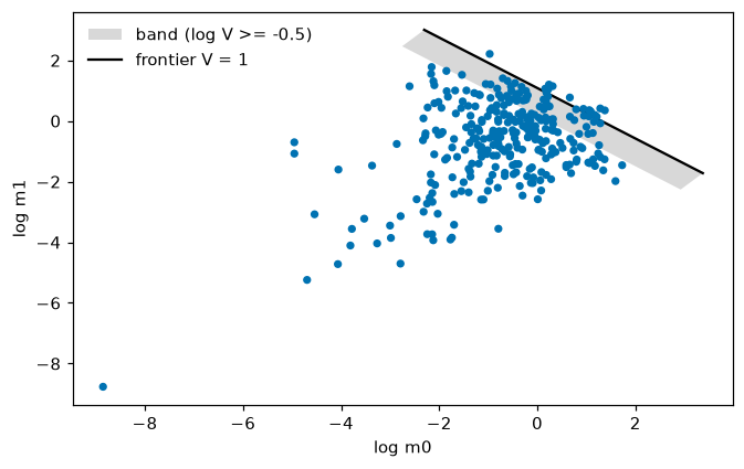
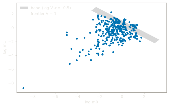
The idea is easiest to see with two of the metrics, where the model is a line. The grey band is up to 0.5 below the frontier in log V:
from tradespace.plotting import plot_log_plane

X2 = X[:, :2]
ts2 = HyperbolicTradeSpace(temperature=20.0).fit(X2)
plot_log_plane(ts2, X2, band=0.5)
Reading the output
fit learned one exponent per metric, summing to one. report.contending_set lists the metrics that
contend at the edge of the table: here all three, which the report names a
trilemma. report.exponents are the
fitted weights at the fit temperature; their ratios are the elasticities between the contending
metrics, with a minus sign (report.elasticities).
ts.score_samples(X) is the log of V for each design. V, the
invariant value, is a weighted geometric mean of the metrics, 1 on the fitted reference surface, so
its log is negative inside and positive beyond. ts.transform(X) is the chart, d - 1 position coordinates plus that log V, and ts.inverse_transform undoes it.
Your own data
What must hold of your table:
- One row per evaluated design; the evaluation stays outside the package, which never calls your model. Design variables and labels are configuration, not attributes: leave them out (prediction takes them).
- The fit consumes a strictly positive matrix of larger-is-better metrics. Making them so is your
conditioning, with
LogAffinePreconditioner. Zeros are tolerated, negatives rejected, infeasible rows removed first. - The exponents describe the conditioned metrics of your sample, not the system's Pareto boundary, its best trade-offs (limitations).