Fitting
HyperbolicTradeSpace fits the frontier model to conditioned metrics. At one term it solves a convex
problem and returns the minimizer.
One term
from tradespace import (
    HyperbolicTradeSpace,
    make_frontier_data,
)

X, info = make_frontier_data(300, 3, random_state=0)
ts = HyperbolicTradeSpace(temperature=20.0).fit(X)
print(ts.exponents_.round(2), round(ts.frac_above_, 2))
The fitted values to read first:
exponents_: shape(n_terms, d), each row non-negative and summing to one.frac_above_: the fraction of designs beyond the surface V = 1.n_eff_: how many designs carry the fit.loss_andmean_slack_:loss_is what the solver minimized, the soft maximum at one term and the mean slack at several, so it is not comparable across numbers of terms.mean_slack_is the mean shortfall below the fitted reference surface, defined at every number of terms; compare fits with it, at a fixed temperature.- The chart's basis, offsets and support weights are
basis_,log_offset_andsupport_weights_.training_log_v_is log V of the training rows. termination_andconditioning_: how the fit stopped and how well its exponents are identified (termination page).
Keep min_exponent (a floor on every exponent) at 0 to
read the contending set, and choose coordinates as "ilr" or "alr", the isometric and additive log-ratio bases.
Choosing the temperature
temperature is tau, how hard the maximum is. Infinity (np.inf) is the exact maximum. It gives the supporting
envelope, with no design above it. A finite tau gives the fitted
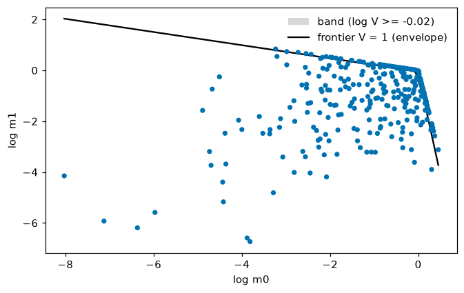
reference surface and a few designs beyond V = 1. The near-frontier band is the designs with |log V| below 1/tau.
select_temperature picks tau so that a target fraction of designs lies above V = 1:
from tradespace import (
    make_frontier_data,
    select_temperature,
)

X, info = make_frontier_data(300, 3, random_state=0)
tau = select_temperature(X, target_frac_above=0.35, bounds=(3, 1e4))
print(round(tau, 1))
This table has 30 percent of its rows on the planted frontier, hence the target 0.35;
for real data start at the default 0.10 with bounds=(3, 1e4). If that raises "not bracketed", raise the target or the upper bound, as the message says. The result is a tau within tol, the accepted error in frac_above_, of the target, so on an exact-relation table it moves with the bounds. Use tau of 3 and above; below it
frac_above_ is not monotone. The fit temperature draws the fit against tau.
Several terms
One term is flat in log space, with constant elasticities. When the rates vary by region, fit
n_terms=K terms, where you choose K (Choosing K):
from tradespace import (
    HyperbolicTradeSpace,
    make_frontier_data,
)

X, info = make_frontier_data(400, 4, n_terms=3, random_state=0)
ts = HyperbolicTradeSpace(
    n_terms=3, temperature=50.0, random_state=0
).fit(X)
print(ts.exponents_.shape, ts.termination_.status)
Fitting alternates weights from the current model with a refit. It starts from n_restarts seeds
and keeps the best. assign_cells(X) reads the cell of new
rows. Options:
term_temperature(kappa, term temperature, default infinity): infinity, one label per design; finite, every design weighs every term. Read kappa on the scale of tau: far below it, terms merge. At tau = 50, kappa = 5000 is within 0.001 of the infinite-kappa exponents.term_aggregation:"sum"(default) or"mean", which subtracts log K / kappa; with the sum, a repeated term shifts the soft maximum by log 2 / kappa.penalty="reweighted_l1"withalphapushes small exponents to exact zero, at finite temperature only.refit_stepis"support"(default) or"tangent", which is not monotone and is never reported as a local optimum.
cell_ gives each training row's cell; coefficients_ and term_share_ the terms' coefficients
and term shares. At one term cell_ is all zeros and term_share_ is
[1.0]. Terms are ordered by term share, largest first (ties by cell size, then the first metric's
exponent); every per-term attribute follows.
The temperature and the band at several terms
With several terms the term planes are not supporting planes, so frac_above_ levels off above
zero as tau grows and the default target 0.10 raises "not bracketed". Choose a target above the
level-off.
trade_off_report takes its band from the temperature, 1/tau. A term whose cell has fewer than
min_near_frontier designs in the band raises. The message names the band that holds enough
designs and the matching temperature.
from tradespace.plotting import plot_log_plane

X2, _ = make_frontier_data(300, 2, n_terms=3, random_state=0)
ts2 = HyperbolicTradeSpace(
    n_terms=3, temperature=50.0, random_state=0
).fit(X2)
plot_log_plane(ts2, X2)
Synthetic data
make_frontier_data plants a frontier, with n_terms=K for K terms; make_configured_frontier_data
also returns configuration variables.