The chart, white space and plots
A fitted model gives every design two kinds of coordinate. One is log V, the level offset
to the fitted reference surface: negative inside, positive beyond. The other d - 1 say where along the surface the design sits,
free of overall scale. Together they are a reversible rewriting of the metrics.
import numpy as np
from tradespace import (
    HyperbolicTradeSpace,
    make_frontier_data,
)

X, info = make_frontier_data(300, 3, random_state=0)
ts = HyperbolicTradeSpace(temperature=20.0).fit(X)
# columns: Z (d - 1 of them), then log V
chart = ts.transform(X)
Z, log_v = chart[:, :-1], chart[:, -1]
print(
    np.allclose(ts.inverse_transform(chart), X),
    np.allclose(ts.score_samples(X), log_v),
)
transform returns the chart, inverse_transform inverts it, and score_samples is log V alone. A
row with a zero metric has nan coordinates and no inverse.
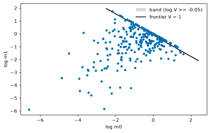
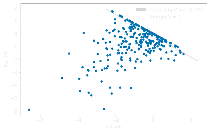
With two metrics the chart is the log plane itself:
from tradespace.plotting import plot_log_plane

X2, _ = make_frontier_data(300, 2, random_state=0)
ts2 = HyperbolicTradeSpace(temperature=20.0).fit(X2)
plot_log_plane(ts2, X2)
Reading log V
V is a factor of improvement: doubling every metric doubles V.
invariant_value(X)returns V.project(X)returns the design moved onto V = 1 by scaling all its metrics together.improvement_factors(X)gives, per metric, the factor on that metric alone that reaches V = 1 (infwhere the exponent is numerically zero).
At a finite temperature some training designs lie beyond V = 1 by construction. A score is
meaningful relative to the near-frontier band, |log V| below 1/tau. Compare tau * log V and the rank of log V among
training scores, not V - 1 alone. A score beyond the surface is not a verdict that the design is
good.
For a multi-term fit, log V is the maximum over terms at the default term_temperature=inf, and
improvement_factors uses each row's assigned term.
White space
Regions of the position coordinates that no design occupies are white space. The functions below find them:
knn_gap_scores(Z, k=5): mean distance to the k nearest neighbours, normalized by its median.find_holes(Z, resolution=50, threshold=2.0): grid points inside the convex hull of Z that sit far from every design; supportsd - 1of 1, 2 or 3.frontier_targets(Z_points, estimator, preconditioner=None): sets log V = 0 at given positions and maps back to metrics and, with a preconditioner, to attributes.orient_by_pca(Z, mask=None): rotates to the principal axes of the masked rows.
The white space of a three-metric fit, most isolated first:
from tradespace.gaps import find_holes

X3, _ = make_frontier_data(300, 3, random_state=0)
ts3 = HyperbolicTradeSpace(temperature=20.0).fit(X3)
chart3 = ts3.transform(X3)
holes, scores = find_holes(chart3[:, :-1], resolution=30, threshold=3.0)
print(len(holes), scores[:3].round(2))
White space is a candidate and not a verdict. An empty region can be an opportunity, a categorical stratum that cannot be occupied, or unsampled. The score cannot tell these apart; you decide. The surface is also convex in log space, so structure that is not convex there is invisible to it.
Plots
tradespace.plotting provides six plots:
plot_log_plane: two metrics, the data, the frontier and its band.plot_frontier_surface_3d: three metrics, the frontier surface.plot_frontier_coordinates(Z, log_v): the chart, the columns ofts.transform(X), with optional white space and targets.plot_v_by_variable: log V against a configuration variable.plot_association: the association among near-frontier designs, from the trade-off report, as a heatmap.plot_ternary: three metrics as shares of a total, with the region each term dominates (example);ternary_marker_valuesgives V at its markers.
Each accepts an optional ax and returns a matplotlib Axes; nothing calls plt.show(). The designs are one colour by default, whatever the number of terms. In
plot_log_plane and plot_frontier_surface_3d, color="cell" colours them by cell, the term that
scores each highest (cell_labels(estimator, X)). Any other string raises ValueError.