Reading trade-offs and tensions
trade_off_report(estimator, X) returns a frozen TradeOffReport that says which metrics contend and
how they trade. The model looks for the binding constraint, so the report describes a trade-off, where
principal component analysis would describe spread.
from tradespace import (
    HyperbolicTradeSpace,
    make_frontier_data,
    trade_off_report,
)

X, info = make_frontier_data(300, 3, random_state=0)
ts = HyperbolicTradeSpace(temperature=20.0).fit(X)
report = trade_off_report(ts, X)
print(report.contending_set, report.n_lemma, report.lemma_name)
print(report.elasticities.round(2))
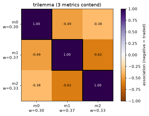
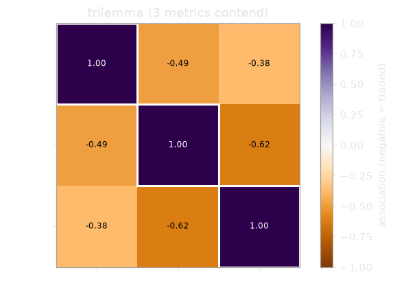
plot_association draws the report as a heatmap:
from tradespace.plotting import plot_association

plot_association(report, names=["m0", "m1", "m2"])
The contending set and the n-lemma
contending_set holds the metrics with positive exponent in the exact-maximum fit (tau = infinity,
exponents above 1e-9). contending_exponents are their exponents, n_lemma is the set's size and lemma_name names it. The names are monolemma, dilemma,
trilemma, then an n-lemma. n is read from the fitted exponents, not chosen before the fit. Read contending_exponents before the name. The report solves the tau = infinity program itself, independent of the
fit temperature. min_exponent must be 0 for this reading, because a positive floor masks the
sparsity. The report warns when the estimator was fitted with a floor.
Participation and elasticities
At the fit temperature the exponents are smoothed, so a small one means weak participation, not
membership. participating marks metrics whose exponent exceeds the participation threshold
(threshold, default 1e-3); an exponent at or below 1e-12 is numerically zero. elasticities[j, k]
is the percentage change of metric j per percentage change of
metric k along the surface. It is constant within a term and nan where metric j does not participate. It
describes a feature of the fitted model, not a causal exchange.
Association among near-frontier designs
For designs with absolute log V below band,
association is the Pearson or Spearman correlation of the log-metrics. Negative is traded, positive
is aligned; association_kind says which. The band is 1/tau by default, or 0.1 at infinite tau, and n_near_frontier counts the designs in it. Near the surface the weighted sum of log-metrics is almost constant, so a binding
constraint produces negative association even where no designer traded the metrics (closure_note
says so).
Spread directions
Three fields describe the spread of the near-frontier designs along the surface:
spread_directions: the principal directions of the near-frontier chart coordinates.spread_loadings: the same directions as loadings on the log-metrics.explained_spread: the share of variance along each.
They equal orient_by_pca on the same rows.
The tension matrix
The elasticity is the same at every point of a term; the tension is not. It is the derivative of
one metric along the term as another rises, the others held: T[i, j] = -(w_i / w_j)(m_j / m_i).
tension_matrix gives each term's matrix at the term's balanced point, from the fit;
design_tensions gives each design's own, from the data.
from tradespace import design_tensions, tension_matrix

T = tension_matrix(ts, X)
print(T.shape, T[0].round(2))
dt = design_tensions(ts, X[:2])
print(dt.term, dt.tensions[0].round(2))
A cell is negative where both metrics carry an exponent on the term, 0 where only the row metric
carries none, and nan (blank, not zero) where the column metric carries none. At K > 1 by_term
reports the other terms' values beside a design's own, never merged. A tension is a rate along the
surface with the other metrics held, not the effect of changing a design variable
(routes back).
With several terms
At K > 1 the function returns a list of K reports, one per term, each on the rows of that term's
cell. A term whose cell (at K = 1, all rows) has fewer than min_near_frontier (default 10) near-frontier rows raises
ValueError; widen band or lower min_near_frontier.
A cap can hide a slope
A term reported as a monolemma is a cap: one metric binds on the rows of its cell. It does
not say the design space has no trade-off. Here the planted frontier is flat for low m0 and falls
beyond, and the tail has few rows:
import numpy as np

rng = np.random.default_rng(0)
a = rng.uniform(-3, 0.5, 300)
b = np.minimum(0, -a) - rng.exponential(0.1, 300)
Xc = np.exp(np.c_[a, b])
one = HyperbolicTradeSpace(temperature=np.inf).fit(Xc)
two = HyperbolicTradeSpace(
    n_terms=2, temperature=50.0, random_state=0
).fit(Xc)
reports = trade_off_report(two, Xc)
print(round(one.mean_slack_, 3), round(two.mean_slack_, 3))
print([r.lemma_name for r in reports])
assert "monolemma" in [r.lemma_name for r in reports]
assert two.mean_slack_ < one.mean_slack_ / 3
One term blends cap and slope into a dilemma that fits neither. Two terms return the cap and the slope as separate terms, at a fraction of the mean slack (0.043 against 0.351).
What it cannot say
Each report describes one term and so one trade-off. It depends on the band and is a statement about the sampled table. Trade-offs the sampling never exercised cannot appear. Whether a contending set is a recognizable dilemma is for the engineer to decide.