The fit temperature
The fit temperature tau sets how hard the maximum is (definition). A table fitted at one tau is one point on a path from tau near zero to infinite tau.
Draw the path
Select tau by the convention (Fitting), fit, then sweep.
temperature_path refits at each temperature of a sweep, twelve log-spaced values from 3 to 1000
with the fit temperature among them, then infinity. plot_temperature_path draws it. Use tau of 3
and above.
import numpy as np
from tradespace import (
    HyperbolicTradeSpace,
    make_frontier_data,
    select_temperature,
)
from tradespace.plotting import (
    plot_temperature_path,
    temperature_path,
)

X, info = make_frontier_data(
    300,
    5,
    exponents=[0.45, 0.3, 0.15, 0.1, 0.0],
    noise=0.05,
    random_state=0,
)
tau = select_temperature(X, 0.10, bounds=(3, 1e4))
ts = HyperbolicTradeSpace(temperature=tau, random_state=0).fit(X)
path = temperature_path(ts, X)
print(round(tau, 1), round(ts.n_eff_, 1))
print(np.round(path["exponents"][[0, path["fit_index"], -1]], 3))
plot_temperature_path(ts, X)
Three readings
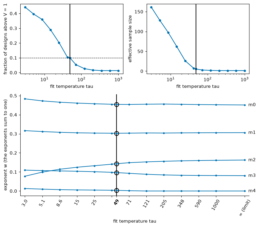
A metric enters or leaves the support. An exponent is non-negative, so it can rest at zero. The fifth metric has a small exponent at low tau and falls to numerically zero between tau of 83 and 88, and stays there up to infinity. That is a change of support: one metric leaves the set of metrics the fit uses. The same shape is the kink of a lasso regularization path, where a coefficient reaches zero at a penalty weight. It is an analogy: tau is how soft a maximum is, not a penalty weight on the exponents. The change is sometimes called a "phase transition"; here it means only this change of support.
Some exponents hold and some move. The contending set is the support at infinite tau (the n-lemma's members): here the first four metrics. Their exponents move by less than 0.09 across the whole sweep, with the largest move in the third. The fifth metric participates at the fit temperature (its exponent is above the participation threshold of 0.001) but is outside the contending set: the softness of the maximum holds it in.
The price is effective sample size. Raising tau leaves fewer designs carrying the fit. Here
n_eff_ is 162 at tau = 3 of 300 designs, 5.3 at the convention's fit temperature and 1.3 at
infinity. The convention, 10 percent of designs above V = 1, is one point on that trade. Move it by
the target:
for target in (0.05, 0.10, 0.20, 0.30):
    t = select_temperature(X, target, bounds=(3, 1e4))
    e = HyperbolicTradeSpace(temperature=t, random_state=0).fit(X)
    print(
        target, round(t, 1), round(e.frac_above_, 2), round(e.n_eff_, 1)
    )
A higher target gives a lower tau, a softer maximum, more designs beyond the fitted reference surface and more designs carrying the fit. Choose the target you can defend from the path: exponents that hold across the temperatures you could have chosen, and an effective sample that is more than a handful of designs.
The two ends
tau to infinity. The maximum is exact, no design lies above the surface, and the fit is the supporting envelope (lemma 5 in Appendix E). The last position of the path is this limit.
tau to zero. The small-tau end is a regularity the sweep shows, not a derived limit. What is
derived is that the soft maximum tends to the mean of the scores, so the weights become uniform and
n_eff_ tends to the number of designs, and that on centred log-metrics, whose mean score is zero,
the first term that depends on the exponents is tau over two times the variance of the score
(lemma 22 in Appendix E). Whether the exponents tend to the combination of least variance on the simplex is
not proved: the lemma does not bound the remainder over the simplex.