Perovskite solar cells
Where the devices come from
The Perovskite Database Project extracted the metal-halide perovskite solar cells reported in peer-reviewed papers into one open table 1. Version 1.0.1 (doi:10.5281/zenodo.5837035, licence CC BY 4.0, credited to that paper) holds 42,443 devices in 410 columns. A row is one reported device. The fetch downloads the 3.3 MB archive, stops if its size or hash differs from manifest.toml, then fits and writes results.json.
uv run python examples/perovskite/run.py
The attributes
attribute  meaning                       unit     column          orient
Voc        open-circuit voltage          V        JV_default_Voc  +1
Jsc        short-circuit current density mA/cm2   JV_default_Jsc  +1
FF         fill factor: delivered power  fraction JV_default_FF   +1
           over Voc times Jsc
set aside: PCE, power conversion efficiency (JV_default_PCE), the
           product of the three over the input power
All three come from the current-voltage scan the authors called default. Rows with a missing, zero or negative attribute, or FF above 1, are dropped, leaving 40,045.
What the fit is asked
In the detailed-balance limit the band gap sets both the voltage a cell can reach and the current it can collect 2. Among the best reported devices, does Voc trade against Jsc, with a negative association near the frontier, or does the fill factor carry the trade?
The fit
All three are larger-is-better, so nothing is inverted or shifted. Each metric is the log of its attribute divided by its spread (the standard scaler), so one fit temperature means the same for the three. Without a scaler, FF, whose log varies least, takes 0.99 and the Voc-Jsc association turns positive (+0.29).
The fit temperature is 18.8, chosen so that a tenth of the rows lie above the fitted surface. At K = 2 the same temperature gives term shares of 0.976 and 0.024 and a mean slack of 0.560 against 0.594 at K = 1. The small term holds 2.4 percent of the rows and puts Jsc's exponent at 0.
import sys

sys.path.insert(0, ".")
from examples.perovskite import run
from tradespace import (
    HyperbolicTradeSpace,
    select_temperature,
)
from tradespace.plotting import plot_ternary

M = run.condition(run.feasible(run.load()))
tau = select_temperature(M, 0.10, bounds=(3, 1e4))
fit = HyperbolicTradeSpace(temperature=tau, random_state=0).fit(M)
plot_ternary(fit, M, names=run.NAMES, lines=True)
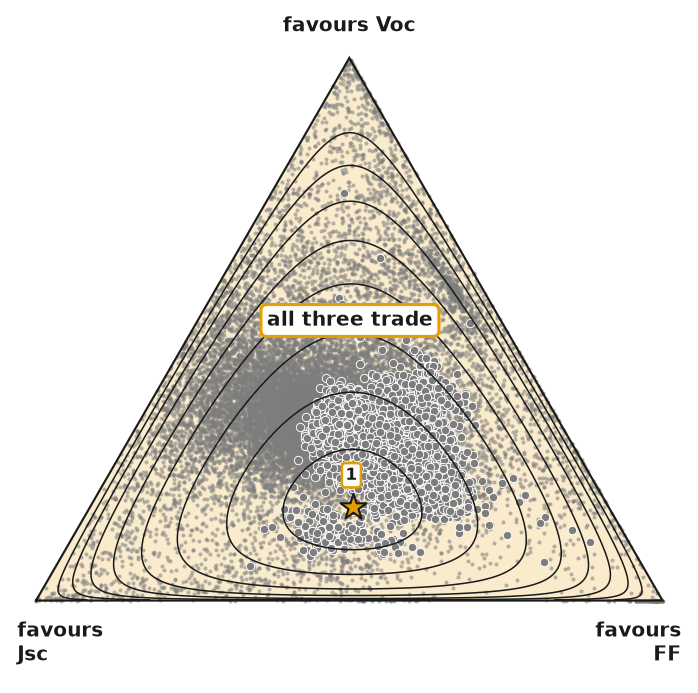
Voc, Jsc and FF are all in the contending set, so the n-lemma is 3. Across the standard scaler, the robust scaler, the quantile map and the cap on five rows, each exponent moves: Voc from 0.12 to 0.43, Jsc from 0.27 to 0.75, FF from 0.02 to 0.61. The near-frontier association of Voc with Jsc is negative in all four, from -0.13 to -0.82. Jsc with FF is negative in all four (-0.27 to -0.64), and Voc with FF is negative in three (-0.39 to -0.44) and +0.23 under the cap. In the standard-scaler fit the strongest pair is Jsc with FF (-0.63), not Voc with Jsc (-0.14).
The extremes. An exact maximum is set by the largest rows. Five rows have Voc above 2 V or Jsc above 40 mA/cm2, probably module or unit entries. Capping them moves the Voc-Jsc association from -0.14 to -0.82. Cap or remove entries that cannot be real, refit, and state the cap.
A derived metric. Added as a fourth metric, power conversion efficiency (PCE) takes exponent 0.50 and FF falls to 0.00: a derived metric absorbs the attributes it summarizes.
The check on your own dataset. Refit with one conditioning choice changed. If the contending set or a sign of the near-frontier association moves, the choice decided the result, and the analysis states it.
from tradespace import (
    HyperbolicTradeSpace,
    trade_off_report,
)

fit = HyperbolicTradeSpace(temperature=tau).fit(M)
report = trade_off_report(fit, M)
report.contending_set, report.association, fit.exponents_
What the fit says
Near the frontier of reported devices, voltage is gained at the cost of current under every conditioning choice: the pair the detailed-balance limit names is traded. It is not the only trade, nor the strongest in the standard-scaler fit, and its size depends on five suspect rows. All three metrics contend in each of the four conditioning fits, so the signs carry the reading, not the set or one exponent.
What the example cannot show
The frontier is the field's published best, not a physical limit: publication favours efficient devices, and a few thousand papers supply the rows. The band gap is not a metric, so the fit cannot say the gap moves a device along the trade. No decision-maker is posed on the dataset, so it has no objectives, and the default scan is whichever scan the authors called default.
-
T. Jesper Jacobsson, Adam Hultqvist, Alberto García-Fernández, and others. An open-access database and analysis tool for perovskite solar cells based on the FAIR data principles. Nature Energy, 7(1):107–115, 2021. doi:10.1038/s41560-021-00941-3. ↩
-
William Shockley and Hans J. Queisser. Detailed balance limit of efficiency of p-n junction solar cells. Journal of Applied Physics, 32(3):510–519, 1961. doi:10.1063/1.1736034. ↩